TAFE NSW coursework
Thermofluid models
Modelled pipeline pressure drop, heat-exchanger energy balance, and vacuum-system energy demand in Excel.
What I did
- Used Goal Seek for the pipeline flow, Solver for the heat-exchanger flow rates and outlet temperatures, and the analytical isothermal-work equation for the vacuum system.
- Ran sensitivity cases: pipeline flow rate against pressure drop, heat-exchanger flow rates against outlet temperatures, and the vacuum system’s target pressure against pressure ratio and work.
- Rebuilt the three models in JavaScript for this page.
Models
Pipeline pressure drop
Calculated the optimal flow rate for a 100 m pipeline of 0.5 m bore carrying oil at 0.1 m³/s. Used the Darcy–Weisbach equation with the laminar friction factor to find how much pressure was lost to wall friction along the pipe at varied flow rates.
- Reynolds number
- 2165 (laminar)
- Pressure drop
- 651.9 Pa
- Head loss
- 0.0783 m
● Current □ Optimal
Heat exchanger
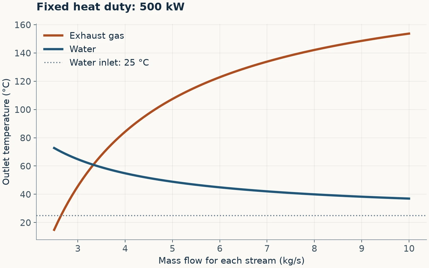
Calculated the flow rates for a process that needed 500 kW transferred from hot exhaust gas to water, cooling the gas and warming the water without the two streams mixing. Each stream followed the steady-flow energy balance Q̇ = ṁcₚΔT at the fixed duty.
- Water outlet temperature
- 50.09 °C
- Gas outlet temperature
- 69.99 °C
Water · Gas — outlet temperature versus mass flow
● Current □ Optimal
Vacuum system
Calculated the minimum energy needed to evacuate a 1 m³ chamber from atmosphere to 0.01 atm (1.013 kPa), where it was held for a manufacturing process. The model showed that the energy demand climbed steeply as the target pressure fell, so specifying no deeper a vacuum than the process required was the biggest energy saving available.
- Pressure ratio
- 100 : 1
- Isothermal work
- 466.5 kJ
● Current □ Optimal